Difference between revisions of "Quick Look Tool"

Revision as of 01:56, 12 December 2016

SpUpNIC Quick Look Reduction Tool

Introduction

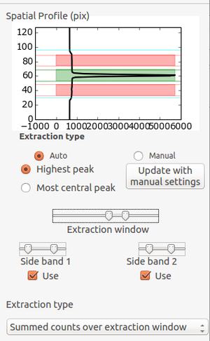
The Quick Look tool is designed to allow users to quickly assess the quality of their data. It automatically produces simple 1D extractions of science data with a reasonable guess for the target of interest (selectable as either the highest peak or the most central peak in the spatial direction); attempts a sky subtraction using two sidebands (which will also subtract the bias from the raw frame), and produces a 1D extraction.

For arcs, automatic wavelength calibration is attempted. The accuracy of this is appropriate for the spirit of a quick look tool and is typically ~2A. This allows the observer to check that the wavelength range of interest is being covered and to identify spectral features in science spectra. This is not intended to be a final science-quality level reduction and there are a number of caveats on the extraction and calibration process listed below. However, for some users, this may be entirely sufficient for their science needs. Even if it is not precise enough, it can be used as a starting point for a more careful reduction and notes on this are given below.

Change Log

Quick Start

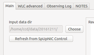
• At the start of a new night of observing, press the "Refresh from SpUpNIC Control" button. This updates the data directory where the QL looks for new data.

• As a new image is written to disk from the observing GUI (SpUpNIC Control), it will appear in the QL window. Each image will appear as the 2D raw image (upper panel) and a 1D extraction (lower panel). More details of how this is done are given below.

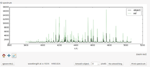
• If an arc is found, the QL tool will attempt an automatic wavelength calibration and plot the calculated wavelength scale on the image. The accuracy of this solution can be easily seen by comparing with the library reference arc (green spectrum) plotted over the top.

• If a science frame is found, the wavelength scale shown will be taken from the previous arc. NOTE: there is no checking that the previous arc is for the same target/configuration as the science frame. It is simply assumed that the observer will always take an arc prior to a science exposure.

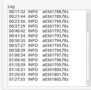
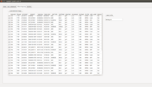
• As new data rolls in, it is added to the Observing Log (accessible under the tab of the same name). This will provide a summary of the most useful header keywords for each image. This may be written to a file at the end of the night to produce a record of all the data produced. It is also possible to click anywhere in the row on any of the images listed in the log and reload the image in the QL tool.
  • Useful trick: if you want to apply a wavelength solution of an arbitrary arc to a science frame, simply load the arc followed by the science frame. Frames may also be loaded by typing the name in the "Current Frame" box and clicking update.

• For each frame, a 1D extraction in both ascii and FITS format is automatically written to a subdirectory, redux/, of the input data directory.

Layout

Input data directory

2D spectrum view

Profile Pane

1D spectrum view

GUI log

Observing Log Tab

Advanced config

To edit the bounds of the 2D spectrum (cyan lines in 2D plot window) edit as root the following file: /usr/local/etc/qlgui/pars.json The upper and lower bounds of the slit (which can be read off the 2D plot window using the cursor) are given by sl0 and sl1 respectively for the given grating name. e.g. for grating 5, the upper and lower bands are gr5_sl1 and gr5_sl0. Edit the numbers appropriately and resave the file. The changes should take effect the next time a spectrum is loaded.